
初めに
本記事は Random Forest と Isolation Forest について記載しています。
機械学習に関連する他の記事は以下をご覧ください。
■機械学習のアルゴリズム
■ディープラーニング
- 【ディープラーニング入門1】AI・機械学習・ディープラーニングとは
- 【ディープラーニング入門2】パーセプトロン・ニューラルネットワーク
- 【ディープラーニング入門3】バックプロパゲーション (誤差逆伝播法)
- 【ディープラーニング入門4】学習・重み・ハイパーパラメータの最適化
- 【ディープラーニング入門5】畳み込みニューラルネットワーク (CNN)
ランダムフォレストとは
ランダムフォレストとは、以下の2つのアルゴリズムを利用して、回帰(予測)、分類を行います。
決定木 (decision tree) とは
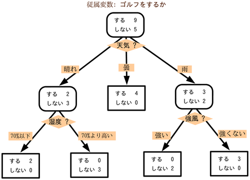
データを分割する基準は、特定のクラス (グループ) を多く含むように分割します。
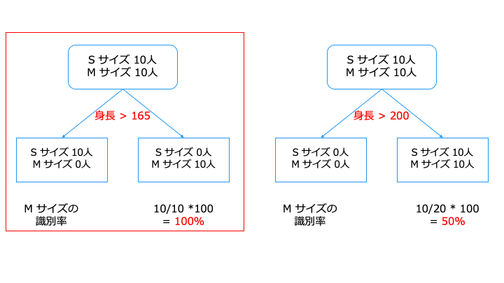
上記の場合、データを分割する基準は、「身長 > 165」の方がいいです。
これは、分割後のノードに1つのクラスが多く含まれているからです。
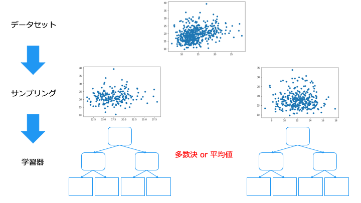
アンサンブル学習の種類
アンサンブル学習は、異なるデータから学習した学習器の方が予測精度が高くなります。
(同じ知識を持つ人だけで多数決をとると、同じ意見しか出ないので多数決の意味ない)
アンサンブル学習では、主に次の4つの手法があります。
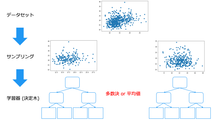
バギング/ブートストラップ・アグリゲーティング

スタッキング
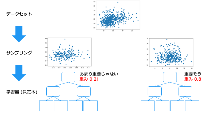
スタッキングは、バギングにおける出来の悪い学習器の結果も同じ重みで評価してしまう問題を解決するものです。
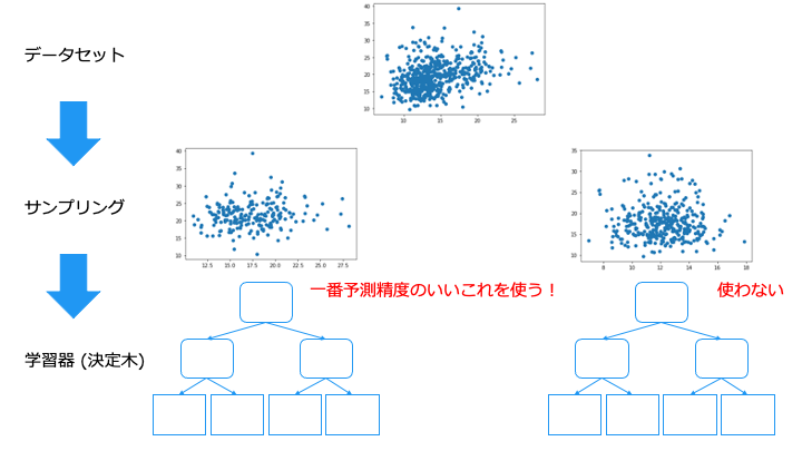
バンピング
バンピングは、外れ値で学習してしまった学習器を捨てることができます。
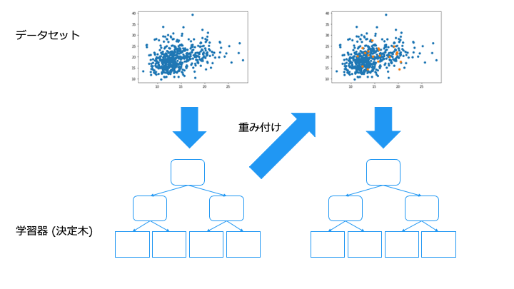
ブースティング
ランダムフォレストのまとめ
これは、異なるデータで学習した学習器を作るためです。(同じような学習器で予測しても同じ予測しか出力されないので多数決の意味がない)
ランダムフォレストの分類を Python + sklearn で実装
ランダムフォレストの分類を Python の sklearn ライブラリで実装してみます。
利用するデータセットは以下です。

ソースコード
from sklearn.ensemble import RandomForestClassifier
from sklearn.datasets import make_classification
from sklearn.model_selection import train_test_split

# データセットを取得
X, y = make_classification(n_samples=1000, n_features=2,
                        n_informative=2, n_redundant=0,
                        random_state=0, shuffle=False)

# データセットの特徴量Xと正解ラベルyを訓練データとテストデータに分ける
X_train, X_test, y_train, y_test = train_test_split(X, y, stratify=y, random_state=0)

# ランダムフォレストで学習
clf = RandomForestClassifier(n_estimators=100, random_state=0).fit(X_train, y_train)

print("予測精度=", clf.score(X_test, y_test)) #テスト用のデータを使って学習器の精度を測る
print("予測結果の詳細\n", clf.predict(X_test)==y_test) #予測結果の正誤を確認
予測精度= 0.956
予測結果の詳細
[ True  True  True  True  True  True  True  True  True  True  True  True
(中略)
  True  True  True  True  True  True  True  True  True  True]
予測精度が 95.6% の学習器が作れました。
学習結果を可視化
学習結果をよりわかりやすくするために、可視化してみます。
import numpy as np
import matplotlib.pyplot as plt
from matplotlib.colors import ListedColormap
from sklearn.ensemble import RandomForestClassifier
from sklearn.datasets import make_classification
from sklearn.model_selection import train_test_split

# 予測の境界線をプロットし可視化
def plot_decision_boundary(model, X, y, margin=0.3):
        _x1 = np.linspace(X[:, 0].min()-margin, X[:, 0].max()+margin, 100) # 0次元目の最小、最大の100分割
        _x2 = np.linspace(X[:, 1].min()-margin, X[:, 1].max()+margin, 100) # 1次元目の最小、最大の100分割
        x1, x2 = np.meshgrid(_x1, _x2)
        X_new = np.c_[x1.ravel(), x2.ravel()]
        y_pred = model.predict(X_new).reshape(x1.shape) # 予測結果
        custom_cmap = ListedColormap(['mediumblue', 'orangered']) # 色の指定
        plt.contourf(x1, x2, y_pred, alpha=0.3, cmap=custom_cmap) # 等高線で境界線を引く

# データセットを取得
X, y = make_classification(n_samples=1000, n_features=2,
                        n_informative=2, n_redundant=0,
                        random_state=0, shuffle=False)

# データセットの特徴量Xと正解ラベルyを訓練データとテストデータに分ける
X_train, X_test, y_train, y_test = train_test_split(X, y, stratify=y, random_state=0)

# ランダムフォレストで学習
clf = RandomForestClassifier(n_estimators=100, random_state=0).fit(X_train, y_train)

plot_decision_boundary(clf, X, y) # 学習結果を可視化
plt.plot(X[:, 0][y==0], X[:, 1][y==0], 'bo', ms=10) # クラス0 のデータを可視化
plt.plot(X[:, 0][y==1], X[:, 1][y==1], "r^", ms=10) # クラス1 のデータを可視化
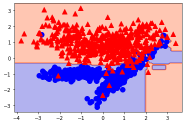
おおよそ分類できていることがわかります。
Isolation Forest とは
Isolation Forest では、以下の2つのアルゴリズムを利用して異常検出を行います。
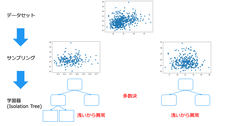
- 学習方法:バギング
- 学習器:Isolation Tree
Isolation Tree のアルゴリズム
Isolation Tree のアルゴリズムは以下のとおりです。

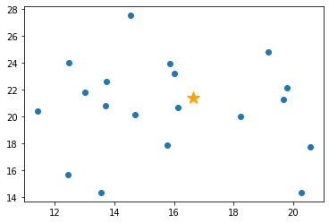
1. 分離するデータポイントを選択
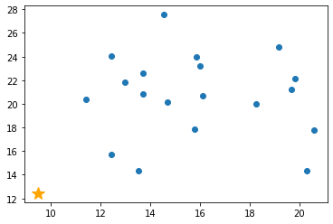
2. ランダムに次元を選択 (今回は x 軸を選択)
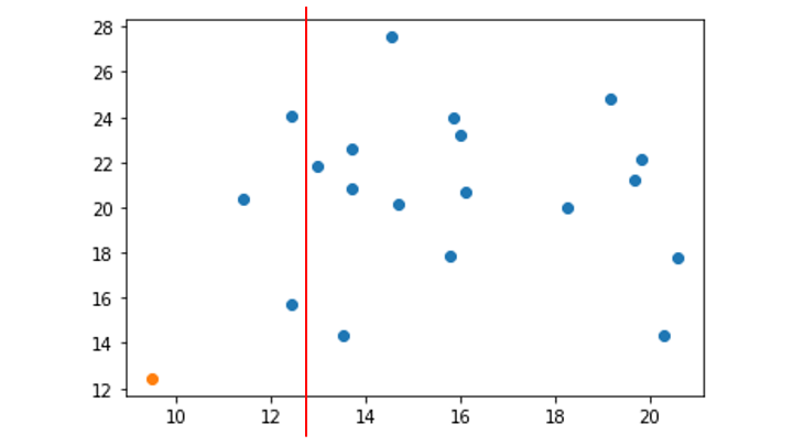
3. 選択した次元の最小値〜最大値の範囲をランダムに選択
今回の場合は x 軸の 9 ~ 21 の間の値をランダムに選択
4. 分離するデータポイントが存在する領域を対象に、データポイントが1つ分離するまで手順2と3を繰り返す
(分離するデータポイントが存在しない領域は無視)
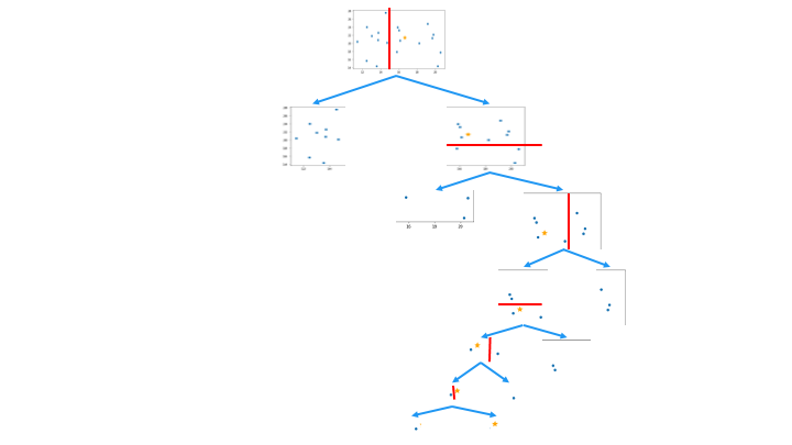
この領域を分割を、木構造で表したものが Isolation Tree です。
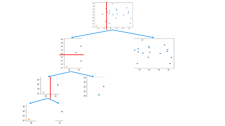
一番上のノードから、分離するデータポイントを持つノードの深さが浅いほど異常 (外れ値) であると判断します。
Isolation Tree を通常値に適用した例 (深さが深くなる)
Isolation Forest のまとめ
Isolation Forest を Python + sklearn で実装
Isolation Forest を Python の sklearn ライブラリで実装します。
利用するデータセットは以下です。

from sklearn.ensemble import IsolationForest
from sklearn.datasets import make_moons

moons = make_moons(n_samples=200, noise=0.05, random_state=0) #学習データ
X_test = np.array([[1, -0.5],[2,1]]) # テスト用データ

# Isolation Forest で学習
clf = IsolationForest(n_estimators=100, random_state=0).fit(moons[0])

print("予測結果\n", clf.predict(X_test)) #1なら正常値、−1なら異常値
plt.plot(moons[0][:, 0], moons[0][:, 1],'o') # 学習用のデータを可視化
plt.plot(X_test[:,0], X_test[:,1], '*', ms=15) # テスト用データの可視化
予測結果
 [ 1 -1]
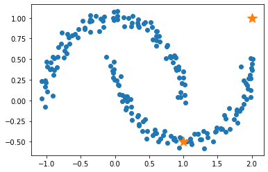
下側の☆が正常値 (1)、右上の☆が異常値 (-1) と判断できていることがわかります。
ランダムカットフォレスト (Random Cut Forest/RFC)
ランダムカットフォレストは Isolation Forest を適用したアルゴリズムです。
次元を選択する際に分散の大きい次元を選択します。(ランダムフォレストはランダムに次元を選択)
The Random Cut Forest (RCF, 2016) method [2] adapted Isolation Forest to work on data streams with bounded memory and lightweight compute.
p.p1 {margin: 0.0px 0.0px 0.0px 0.0px; font: 10.0px Helvetica}
https://opensearch.org/blog/odfe-updates/2019/11/real-time-anomaly-detection-in-open-distro-for-elasticsearch/
RRCF gives more weight to dimension with higher variance (according to SageMaker doc), while I think isolation forest samples at random,.....
https://stackoverflow.com/questions/63115867/isolation-forest-vs-robust-random-cut-forest-in-outlier-detection
もっと詳しく知りたい方は以下をどうぞ
https://proceedings.mlr.press/v48/guha16.pdf機械学習の関連記事
■機械学習のアルゴリズム
■ディープラーニング
- 【ディープラーニング入門1】AI・機械学習・ディープラーニングとは
- 【ディープラーニング入門2】パーセプトロン・ニューラルネットワーク
- 【ディープラーニング入門3】バックプロパゲーション (誤差逆伝播法)
- 【ディープラーニング入門4】学習・重み・ハイパーパラメータの最適化
- 【ディープラーニング入門5】畳み込みニューラルネットワーク (CNN)


参考資料


